Optiwave software can be used in different industries and applications, including Fiber Optic Communication, Sensing, Pharma/Bio, Military & Satcom, Test & Measurement, Fundamental Research, Solar Panels, Components / Devices, etc..
OptiSystem is a comprehensive software design suite that enables users to plan, test, and simulate optical links in the transmission layer of modern optical networks.
OptiSPICE is the first circuit design software for analysis of integrated circuits including interactions of optical and electronic components. It allows for the design and simulation of opto-electronic circuits at the transistor level, from laser drivers to transimpedance amplifiers, optical interconnects and electronic equalizers.
OptiFDTD is a powerful, highly integrated, and user friendly CAD environment that enables the design and simulation of advanced passive and non-linear photonic components.
OptiBPM is a comprehensive CAD environment used for the design of complex optical waveguides. Perform guiding, coupling, switching, splitting, multiplexing, and demultiplexing of optical signals in photonic devices.
OptiFiber The optimal design of a given optical communication system depends directly on the choice of fiber parameters. OptiFiber uses numerical mode solvers and other models specialized to fibers for calculating dispersion, losses, birefringence, and PMD.
Emerging as a de facto standard over the last decade, OptiGrating has delivered powerful and user friendly design software for modeling integrated and fiber optic devices that incorporate optical gratings.
OptiConverge is a collaborative integration framework that seamlessly combines two or more Optiwave products (e.g., OptiSystem, OptiSPICE, OptiFDTD, etc.) and other third party products into unified solutions. Designed to streamline complex workflows, it empowers users to achieve their goals faster by harnessing the collective power of our trusted Optiwave tools.
Inside a dielectric, the time independent Maxwell curl equations with a positive time convention ( ejωt ) are
and the divergence equations are
In the magnetic formulation, the electric field is eliminated from (1) by taking the curl
of the second equation and substituting from the first. For regions of constant permittivity ε , there are no gradients of ε , and the equation simplifies to
In view of the vector identity ∇×∇×A = ∇( ∇ ⋅ A ) – ∇2A , and the property of H having zero divergence, (3) becomes
where is the free space wavenumber.
It is true that it is usually the electric field, and not the magnetic field, that is of interest for applications. The motivation for solving the problem with a magnetic formulation is that the waveguide structure is created by introducing discontinuities in electric permittivity,
ε, and not magnetic permeability, μ . When matching boundary conditions at layer boundaries, the normal component of the electric field is discontinuous, since it is the electric displacement, D= εε0E , and not the electric field that is to be made continuous. Since the permeability is the vacuum level μ0 everywhere, all components of the magnetic field are continuous at all boundaries. The finite difference representation of continuous functions is more accurate than discontinuous functions, and therefore a finite difference formulation based on the magnetic field gives more accurate results than one based on electric fields.
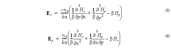
The electric fields are still needed for applications. These fields can be calculated after the fact by taking the curl of the magnetic field (using the second equation in (1)) by finite differences. Explicitly,
In the mode solving problem, the permittivity ε does not vary with z, and so the solution for the magnetic field can be expected to be an harmonic function of z:
and (7) in (4) gives
Since the β is unknown, the mode solving problem is really an eigenvector problem with β2 as the eigenvalue, and the function hx ( x, y ) or hy ( x, y ) as the eigenfunction.