We consider a planar waveguide where x and z are the transverse and propagation directions, respectively, and there is no variation in the y direction ( ∂ ⁄ ∂y ≡ 0 ) .
Furthermore we consider that the planar optical waveguide with width W is surrounded by PML regions with thickness d as shown in Figure 3.
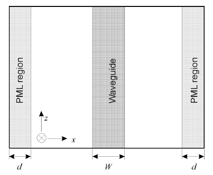
Figure 3: Planar waveguide surrounded by PML
With these assumptions and transversely-scaled version of PML, as defined in “Perfectly Matched Layer (PML)” on page 26, we get the following basic equation from Equation 35:

with
where Ey and Hy are the y components of the electric and magnetic fields respectively, ω is the angular frequency, ε0 and μ0 are the permittivity and permeability of free space, respectively, n is the refractive index, k0 is the free-space wave number, and the parameter s is defined by Equation 45.
We separate the field Φ( x, z ) into two parts: the axially slowly varying envelop term of φ( x, z ) and the rapidly term of exp ( –jk0 nre f z ) . Here, nre f is the reference index.
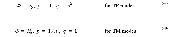
Then, Φ( x, y ) is expressed by
![]()
By substituting Equation 49 into Equation 46, we obtain the following equation for slowly varying complex amplitude φ :
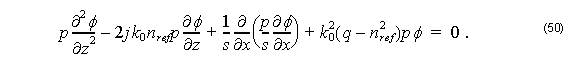
The term ∂p ⁄ ∂z is neglected for TM modes.
Finite Difference Approximant
To obtain the field solution at each cross section we discretise Equation 50 using Finite Differences scheme along x – direction [23] – [27].
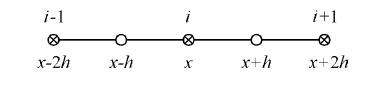
Figure 4: Finite Difference uniform mesh
Formally, we have from Taylor expansion:
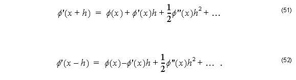
Subtracting Equation 51 from Equation 51 and neglecting higher order terms:
![]()
Thus, for TE modes we get
Here we consider:

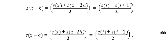
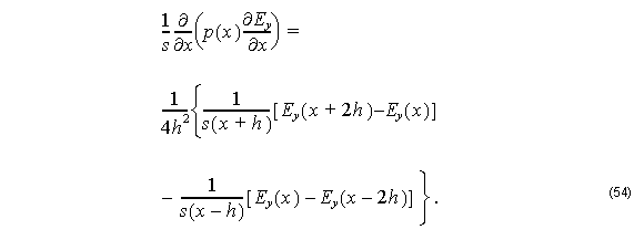
By substituting Equation 55 and Equation 56 into Equation 54, we get:
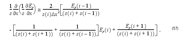
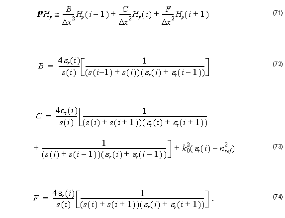
Therefore, we can rewrite Equation 50 for TE modes as

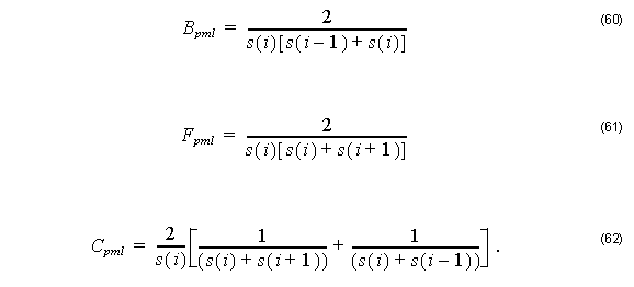
where
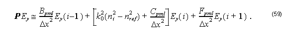
Here,
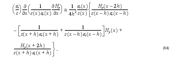
For TM modes we have:
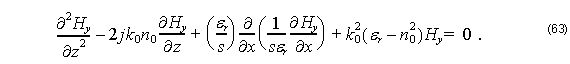
Applying FD scheme in the third term of Equation 63 we obtain:
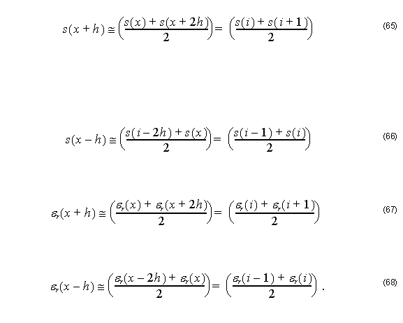
For small h one has:
By substituting Equation 66, Equation 67, and Equation 68 into Equation 64, we get:
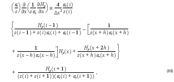
Thus, using FD scheme into Equation 50 for TM modes, we get:

with